
An Interaction or Not? How a few ML Models Generalize to New Data
Source code for this post is here.
This post examines how a few statistical and machine learning models respond to a simple toy example where they're asked to make predictions on new regions of feature space. The key question the models will answer differently is whether there's an "interaction" between two features: does the influence of one feature differ depending on the value of another.
In this case, the data won't provide information about whether there's an interaction or not. Interactions are often real and important, but in many contexts we treat interaction effects as likely to be small (without evidence otherwise). I'll walk through why decision trees and bagged ensembles of decision trees (random forests) can make the opposite assumption: they can strongly prefer an interaction, even when the evidence is equally consistent with including or not including an interaction.
I'll look at point estimates from:
- a linear model
- decision trees and bagged decision trees (random forest), using R's
randomForestpackage - boosted decision trees, using the R's
gbmpackage
I'll also look at two models that capture uncertainty about whether there's an interaction:
- Bayesian linear model with an interaction term
- Bayesian Additive Regression Trees (BART)
BART has the advantage of expressing uncertainty while still being a "machine learning" type model that learns interactions, non-linearities, etc. without the user having to decide which terms to include or the particular functional form.
Whenever possible, I recommend using models like BART that explicitly allow for uncertainty.
The Example
Suppose you're given this data and asked to make a prediction at $X_1 = 0$, $X_2 = 1$ (where there isn't any training data):
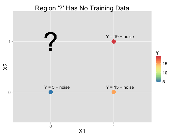
| X1 | X2 | Y | N Training Rows: |
|---|---|---|---|
| 0 | 0 | Y = 5 + noise | 52 |
| 1 | 0 | Y = 15 + noise | 23 |
| 1 | 1 | Y = 19 + noise | 25 |
| 0 | 1 | ? | 0 |
In practice, making an inference at $X_1 = 0$, $X_2 = 1$ would be pretty hopeless. The training data doesn't help much, so your prediction will depend almost entirely on your priors. But that's exactly why I'm using this example to get at what the biases are in various models. Real problems will have elements in common with this example, so it helps get a handle on how models will behave for those problems.
A Linear Model
lmFit <- lm(Y ~ X1 + X2, data = train)
If you fit a linear model of the form $\mathbb{E}[Y] = \beta_0 + \beta_1 X_1 + \beta_2 X_2$, you find
$$\mathbb{E}[Y] = 5 + 10 X_1 + 4 X_2.$$
This fits the training data perfectly and extrapolates to the unseen region of feature space using the assumption that effects are additive.
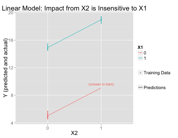
The line for $X_1 = 0$ is parallel to the one for $X_1 = 1$, meaning that the influence of $X_2$ is the same (+4) regardless of the value of $X_1$
Decision Trees (and Random Forest)
Random forests are built from decision trees using an ensembling technique called bagging, which averages a number of independent decision trees. To make the trees different, different trees use different random subsets of the training data. (Additional randomness is usually introduced by allowing each tree to consider a random subset of the features at each split.)
I've fit a random forest and plotted its predictions and the training data. Where there is training data, the model fits that data perfectly (making the same predictions as the linear model), but has decided that $X_2$ only matters when $X_1 = 1$:
rfFit <- randomForest(Y ~ X1 + X2, data = train, mtry=2)
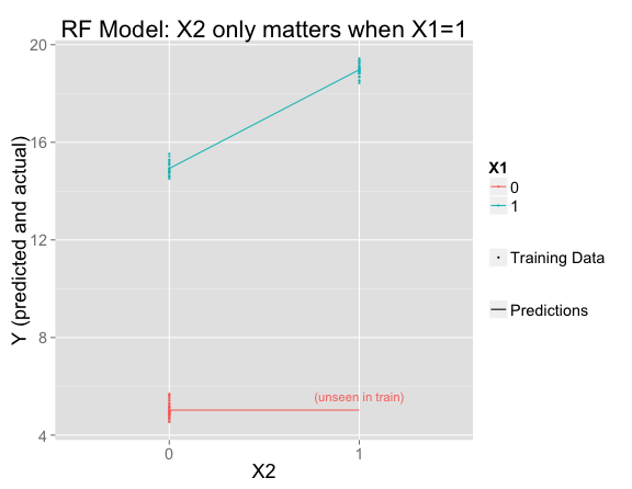
It's easy to understand from the trees why this happened. In this simple example, all of the trees are the same, so it's just as if there were one decision tree. $X_1$ is the most important variable, so first the tree splits on that. Then only the right side splits again on $X_2$ (since the left side has no training set variation in $X_2$):

A couple important settings are:
-
mtry=2means both variables are considered at each split. This choice makes the example clearer, but it also makes sense here becausemtry=2would be the parameter you choose as optimal based on the training data (e.g. through cross-validation). With the default settings, the random forest would fail to replicate even the training data (where there should be no question which predictions are correct). - I'm using the default minimum node size (for regression problems) of 1. If the minimum node size were smaller, it would sometimes happen that a tree doesn't have enough data from one region of feature space to support a split. Even with a minimum size of 1, you would (very rarely) end up working with a random subset of the rows that doesn't represent one region of feature space at all.
Boosted Decision Trees
Boosting is an ensembling technique in which each tree is built based on the residuals from the previous one. Unlike with bagging, this allows the model to add together effects that are each chosen whole controlling for the others, giving the model a bit of an additive charactaristic.
It's possible to represent a well-fitting model as a sum of only two depth-1 trees (this is the same as the linear model):

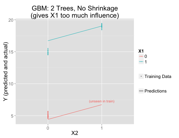
But the gbm can't get to this answer with only two depth-1 trees.
library(gbm)
gbmFit1 <- gbm(Y ~ X1 + X2, data = train, n.trees=2, shrinkage = 1, distribution = "gaussian")
These are (approximately) the trees we get:

| X1 | X2 | Y (mean) | N Training Rows | First Tree Predictions | First Tree Residual |
|---|---|---|---|---|---|
| 0 | 0 | 5 | 52 | 5 | 0 |
| 1 | 0 | 15 | 23 | 17 | -2 |
| 1 | 1 | 19 | 25 | 17 | 2 |
Related to the correlation between $X_1$ and $X_2$ in the training data, the first tree (with a split on $X_1$) assigns too much of the effect to $X_1$ (effect size of $12$ instead of $10$). Then the second tree's split on $X_2$ is based on the residuals from the first (shown in the table above). The residuals for $X_2=0$ (-2 and 0, with roughly twice as much weight on the latter) average to roughly $-\frac{2}{3}$, while the residual on the $X_2=1$ side is roughly $2$.
The second tree has no way to correct the fact that too much signal went into $X_1$ in the first tree. We've fit the two parameters for linear model in two iterations rather than simultaneously.
Instead, boosting generally fits just a small amount of the signal at each stage, making only very small adjustments in the direction of fitting the residuals. This works much better:
library(gbm)
gbmFit2 <- gbm(Y ~ X1 + X2, data = train, n.trees=10000, shrinkage = .01, distribution = "gaussian")
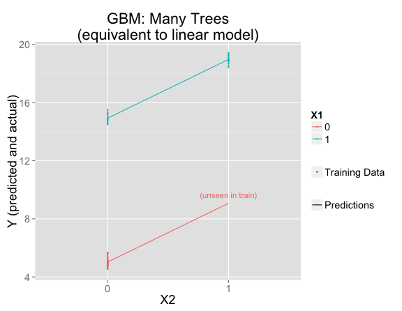
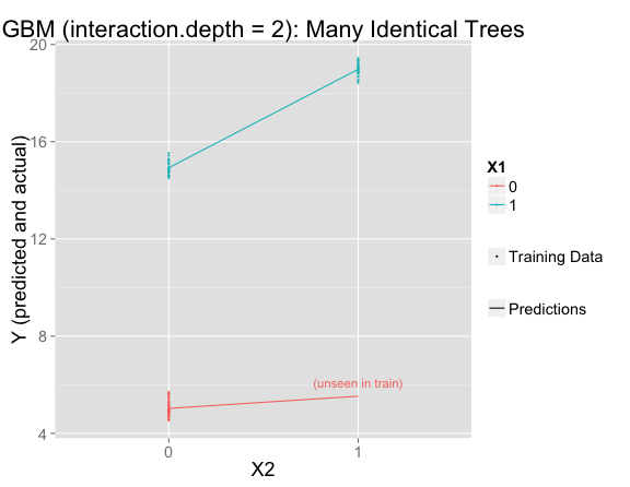
But this is using the default interaction.depth=1, which forces the model to be linear. If interaction.depth=2, the results are similar to if there were only one decision tree:
library(gbm)
gbmFit3 <- gbm(Y ~ X1 + X2, data = train, n.trees=10000, shrinkage = .01, distribution = "gaussian", interaction.depth = 2)
Is it possible for gbm to result in a middle ground between the linear model and the one-tree model? Yes! Two parameters we can tweak for this are:
n.minobsinnode(default: $10$), the minimum number of observations for a leaf node.bag.fraction(default: $0.5$), the number of randomly selected training observations to use for each tree
To get the second (deeper) split, there must be at least n.minobsinnode in each of the smaller groups ($X_1 = 1$, $X_2 = 0$ or $X_1 = 1$, $X_2 = 1$). Increasing n.minobsinnode decreases the number of trees that meet the threshold for a second split:
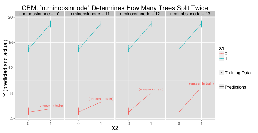
Varying bag.fraction would have a similar effect.
Models with Uncertainty: Linear Regression with Interaction Term
All of the above models deliver point estimates. But really, we should admit to uncertainty about the predictions. Going back to the linear regression, we can add an interaction term to let the model consider interactions. The model is:
$$Y = \beta_0 + \beta_1 X_1 + \beta_2 X_2 + \beta_{12} X_1 X_2 + N(0,\sigma).$$
Without an informative prior distribution, this would be too many free parameters. But I'll put a prior on $\beta_{12}$ (pushing it toward zero). All parameters except $\beta_{12}$ have improper flat priors while $$\beta_{12} \sim N(0,2).$$
Such a simple model doesn't need a flexible tool like Stan, but I like how clear and explicit a model is when you write it down in the Stan language. Stan fits Bayesian models using Markov Chain Monte Carlo (MCMC), so the output is a set of parameter samples from the posterior distribution.
Here's what the model looks like in Stan:
library(rstan)

stanModel1 <- "
data {
int<lower=0> N;
vector[N] X1;
vector[N] X2;
vector[N] Y;
}
parameters {
real beta0;
real beta1;
real beta2;
real beta12;
real<lower=0> sigma;
}
model {
beta12 ~ normal(0, 2);
Y ~ normal(beta0 + beta1*X1 + beta2*X2 + beta12*X1 .* X2, sigma);
}
"
Now instead of one prediction for each point in feature space, we have a set of posterior samples. Each line represents the predictions for one posterior sample, at either $X_1=0$ or $X_1=1$:
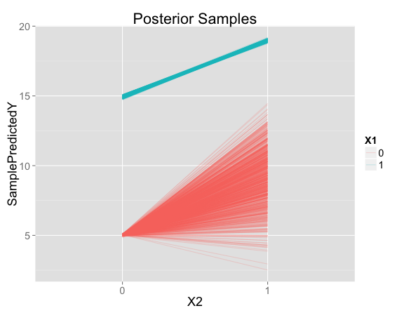
For points like the ones seen in the training data, there is very little uncertainty. But there is a lot of uncertainty about the predicted effect of $X_2$ when $X_1 = 0$.
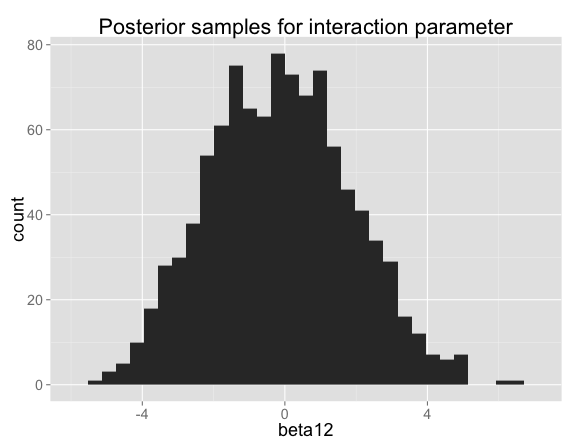
The posterior for the interaction term $\beta_{12}$ is actually very close to the prior (they would be identical with infinite data or no noise in Y), which makes sense because the data don't tell you anything about whether there's an interaction:
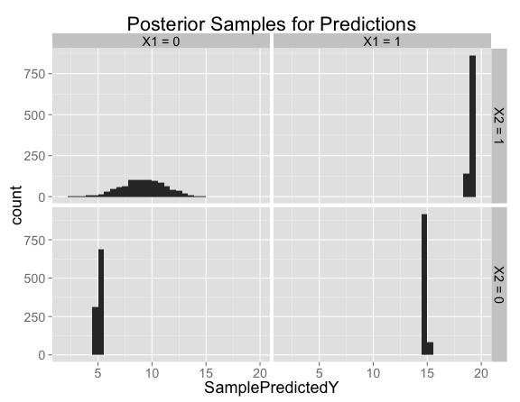
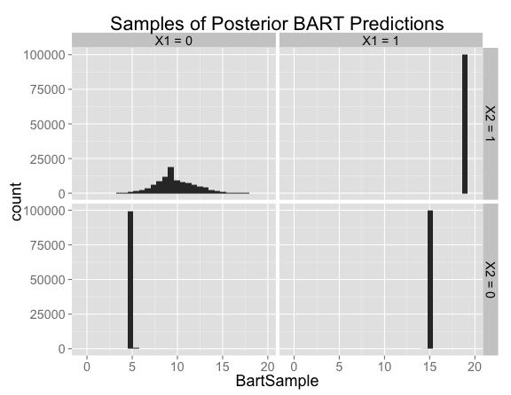
Looking at histograms of posterior samples for predictions is another way to see that there's basically no variation at the points where we have training data:
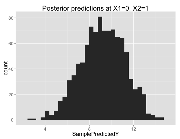
Looking closer at the posterior samples for $X_1 = 0$, $X_2 = 1$, the predictions are centered on 9 (the prediction from our model with no interaction), but has substantial variation in both directions:
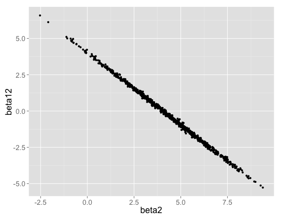
The interaction term can be positive or negative. When the interaction term $\beta_{12}$ is high, $\beta_2$ makes up for it by being low (and vice versa):
Note that if we were to regularize the main effects as well as the interaction term, the predictions at $X_1 = 0$, $X_2 = 1$ would shift to the left. Imagine a prior on $\beta_2$ centered on $0$ as well as the prior already on $\beta_{12}$. In that case, parameters choices with a negative interaction term would be penalized twice: once for the negative $\beta_{12}$, and again for forcing $\beta_2$ higher than it otherwise had to be.
In summary, the Bayesian linear regression (with an interaction term) is appropriately uncertain about predictions in the unseen region of feature space. The particular details of the posterior would depend on how you feel about main effects as compared with to interaction terms: If only the interaction term is pushed toward 0, the predictions are centered around the "no interaction" case. If main effects are pushed toward zero as well, predictions are shifted toward the "positive interaction" case.
Bayesian Additive Regression Trees (BART)
BART is a Bayesian model that's fit using MCMC, so just like with the previous example, we'll get samples from a posterior. The BART model consists of a sum of trees, where we have a prior distribution over the depth of the splits, the values at the leaf nodes, and so on. I don't want to fully describe BART in detail here, so if you're interested have a look at the vignette for the bartMachine R package.
For now, the important thing about BART is that it's a sum of trees, where each tree is fitted in the context of the rest. In the iterative algorithm, each tree is modified one by one based on the residuals from the other trees (unlike random forests, where each tree is independent). This allows BART to better capture additive effects. If the trees all had just one split, we would only capture additive effects.
For example, the linear model above (with no interaction) would be the same as a model that comes from two trees, each with one split: one splitting on $X_1$ and the other on $X_2$.
Trees that are deeper than one split would allow BART to introduce interactions.
library(bartMachine)
nIterAfterBurnIn <- 100000
bartFit <- bartMachine(train[c("X1","X2")], train$Y,
                       num_burn_in=50000,
                       num_trees=10,
                       num_iterations_after_burn_in=nIterAfterBurnIn)
As with all of the previous examples, the model is both correct and confident in the regions where there are training examples.
The predictions in the new region of feature space are similar to the situation we had with the Bayesian linear model with a prior on the interaction term. There's a fair amount of uncertainty, with the posterior distribution centered near the no-interaction case (corresponding to predictions of 9) but allowing positive or negative interactions.
Controlling BART's Settings
To get a sense for how BART's settings affect the inference, consider that the tree depths are controlled by the prior probability of a split occurring at any given node, which is
$$\alpha(1+d)^{-\beta}.$$
The default settings are $\alpha=.95$ and $\beta=2$. This means that BART can allow very deep trees, but deep trees need to overcome this prior against splitting when a node is already deep and so are less common unless the data require them.
In this case, $\beta$ increases, there tend to be more trees with only one split (especially since more splits aren't necessary to explain the training data), leading to a posterior that's more like the no-interaction situation.
BART has other settings that it's good to understand and control them as appropriate, but it can also be used out-of-the-box without thinking too much about those at first.
Implications for Choosing a Model
It helps to be aware of what tendencies your algorithms have. I used a trivial example to demonstrate some tendencies of bagged decision trees (random forests) and boosted decision trees.
This example demonstrates the limits of bootstrapping as an approach to uncertainty. Bootstrapping is a way to get at how your estimates would vary under new samples of the training data. It's especially convenient for bagged estimators, since if you're bagging, you've already done much of the computational work for bootstrapping. But the random forest (and the boosted trees, depending on the parameter settings) doesn't vary with new samples of the training data. This shows that your uncertainty about the truth could be very different from the variation in your model under replicated samples of the training data.
When possible, use methods that explicitly capture uncertainty. I demonstrated adding an interaction term (with an informative prior distribution) to the linear model, as well Bayesian Additive Regression Trees. The former exemplifies a parametric approach where you carefully think about each parameter in the model. The latter is meant to support more "automated" model-building.
Thanks to Dan Becker for pushing me to include GBMs, and to Naftali Harris and Chris Clark for feedback on a draft.